INTELLECTUM VIRTUS
INTELLECTUM VIRTUS
INTELLECTUM VIRTUS
INTELLECTUM VIRTUS
INTELLECTUM VIRTUS
ELECTRICAL ENGINEERING
ELECTRICAL ENGINEERING
ELECTRICAL ENGINEERING
ELECTRICAL ENGINEERING
ELECTRICAL ENGINEERING
KIRCHHOFF’S LAW
KIRCHHOFF’S LAW
KIRCHHOFF’S LAW
KIRCHHOFF’S LAW
KIRCHHOFF’S LAW
FORMULATION
FORMULATION
FORMULATION
FORMULATION
FORMULATION
FORMULATION
FORMULATION
FORMULATION
FORMULATION
 |
|
|
|
|
| In 1845, a German physicist, Gustav Kirchhoff developed a pair or set of rules or laws which deal with the conservation of current and energy within Electrical Circuits. These two rules are commonly known as: Kirchhoff’s Circuit Laws with one of Kirchhoff’s laws dealing with the current flowing around a closed circuit, Kirchhoff’s Current Law, (KCL) while the other law deals with the voltage sources present in a closed circuit, Kirchhoff’s Voltage Law, (KVL). |
| In 1845, a German physicist, Gustav Kirchhoff developed a pair or set of rules or laws which deal with the conservation of current and energy within Electrical Circuits. These two rules are commonly known as: Kirchhoff’s Circuit Laws with one of Kirchhoff’s laws dealing with the current flowing around a closed circuit, Kirchhoff’s Current Law, (KCL) while the other law deals with the voltage sources present in a closed circuit, Kirchhoff’s Voltage Law, (KVL). |
| In 1845, a German physicist, Gustav Kirchhoff developed a pair or set of rules or laws which deal with the conservation of current and energy within Electrical Circuits. These two rules are commonly known as: Kirchhoff’s Circuit Laws with one of Kirchhoff’s laws dealing with the current flowing around a closed circuit, Kirchhoff’s Current Law, (KCL) while the other law deals with the voltage sources present in a closed circuit, Kirchhoff’s Voltage Law, (KVL). |
| In 1845, a German physicist, Gustav Kirchhoff developed a pair or set of rules or laws which deal with the conservation of current and energy within Electrical Circuits. These two rules are commonly known as: Kirchhoff’s Circuit Laws with one of Kirchhoff’s laws dealing with the current flowing around a closed circuit, Kirchhoff’s Current Law, (KCL) while the other law deals with the voltage sources present in a closed circuit, Kirchhoff’s Voltage Law, (KVL). |
| In 1845, a German physicist, Gustav Kirchhoff developed a pair or set of rules or laws which deal with the conservation of current and energy within Electrical Circuits. These two rules are commonly known as: Kirchhoff’s Circuit Laws with one of Kirchhoff’s laws dealing with the current flowing around a closed circuit, Kirchhoff’s Current Law, (KCL) while the other law deals with the voltage sources present in a closed circuit, Kirchhoff’s Voltage Law, (KVL). |
| Resistance can be found when two or more resistors are connected together in either series, parallel or combinations of both, and that these circuits obey Ohm’s Law. However, sometimes in complex circuits such as bridge or T networks, we cannot simply use Ohm’s Law alone to find the voltages or currents circulating within the circuit. For these types of calculations we need certain rules which allow us to obtain the circuit equations and for this we can use Kirchhoff’s Circuit Law. |
| Resistance can be found when two or more resistors are connected together in either series, parallel or combinations of both, and that these circuits obey Ohm’s Law. However, sometimes in complex circuits such as bridge or T networks, we cannot simply use Ohm’s Law alone to find the voltages or currents circulating within the circuit. For these types of calculations we need certain rules which allow us to obtain the circuit equations and for this we can use Kirchhoff’s Circuit Law. |
| Resistance can be found when two or more resistors are connected together in either series, parallel or combinations of both, and that these circuits obey Ohm’s Law. However, sometimes in complex circuits such as bridge or T networks, we cannot simply use Ohm’s Law alone to find the voltages or currents circulating within the circuit. For these types of calculations we need certain rules which allow us to obtain the circuit equations and for this we can use Kirchhoff’s Circuit Law. |
| Resistance can be found when two or more resistors are connected together in either series, parallel or combinations of both, and that these circuits obey Ohm’s Law. However, sometimes in complex circuits such as bridge or T networks, we cannot simply use Ohm’s Law alone to find the voltages or currents circulating within the circuit. For these types of calculations we need certain rules which allow us to obtain the circuit equations and for this we can use Kirchhoff’s Circuit Law. |
| Resistance can be found when two or more resistors are connected together in either series, parallel or combinations of both, and that these circuits obey Ohm’s Law. However, sometimes in complex circuits such as bridge or T networks, we cannot simply use Ohm’s Law alone to find the voltages or currents circulating within the circuit. For these types of calculations we need certain rules which allow us to obtain the circuit equations and for this we can use Kirchhoff’s Circuit Law. |
| Kirchhoff’s Law for Current |
| Kirchhoff’s Law for Current |
| Kirchhoff’s Law for Current |
| Kirchhoff’s Law for Current |
| Kirchhoff’s Law for Current |
| Kirchoff’s Current Law, also known Kirchhoff’s first law, Kirchhoff’s point, junction or nodal rule, states that the algebraic sum of currents at a node is zero. Additionally, the principle of the conservation of Electric Charge implies that: At any node (junction) in an electric circuit , the sum of currents flowing into that node is equal to the sum of currents flowing out of that node, or equivalently: The algebraic sum of currents in a network of conductors meeting at a point is zero. |
| Kirchoff’s Current Law, also known Kirchhoff’s first law, Kirchhoff’s point, junction or nodal rule, states that the algebraic sum of currents at a node is zero. Additionally, the principle of the conservation of Electric Charge implies that: At any node (junction) in an electric circuit , the sum of currents flowing into that node is equal to the sum of currents flowing out of that node, or equivalently: The algebraic sum of currents in a network of conductors meeting at a point is zero. |
| Kirchoff’s Current Law, also known Kirchhoff’s first law, Kirchhoff’s point, junction or nodal rule, states that the algebraic sum of currents at a node is zero. Additionally, the principle of the conservation of Electric Charge implies that: At any node (junction) in an electric circuit , the sum of currents flowing into that node is equal to the sum of currents flowing out of that node, or equivalently: The algebraic sum of currents in a network of conductors meeting at a point is zero. |
| Kirchoff’s Current Law, also known Kirchhoff’s first law, Kirchhoff’s point, junction or nodal rule, states that the algebraic sum of currents at a node is zero. Additionally, the principle of the conservation of Electric Charge implies that: At any node (junction) in an electric circuit , the sum of currents flowing into that node is equal to the sum of currents flowing out of that node, or equivalently: The algebraic sum of currents in a network of conductors meeting at a point is zero. |
| Kirchoff’s Current Law, also known Kirchhoff’s first law, Kirchhoff’s point, junction or nodal rule, states that the algebraic sum of currents at a node is zero. Additionally, the principle of the conservation of Electric Charge implies that: At any node (junction) in an electric circuit , the sum of currents flowing into that node is equal to the sum of currents flowing out of that node, or equivalently: The algebraic sum of currents in a network of conductors meeting at a point is zero. |
 |
|
|
|
|
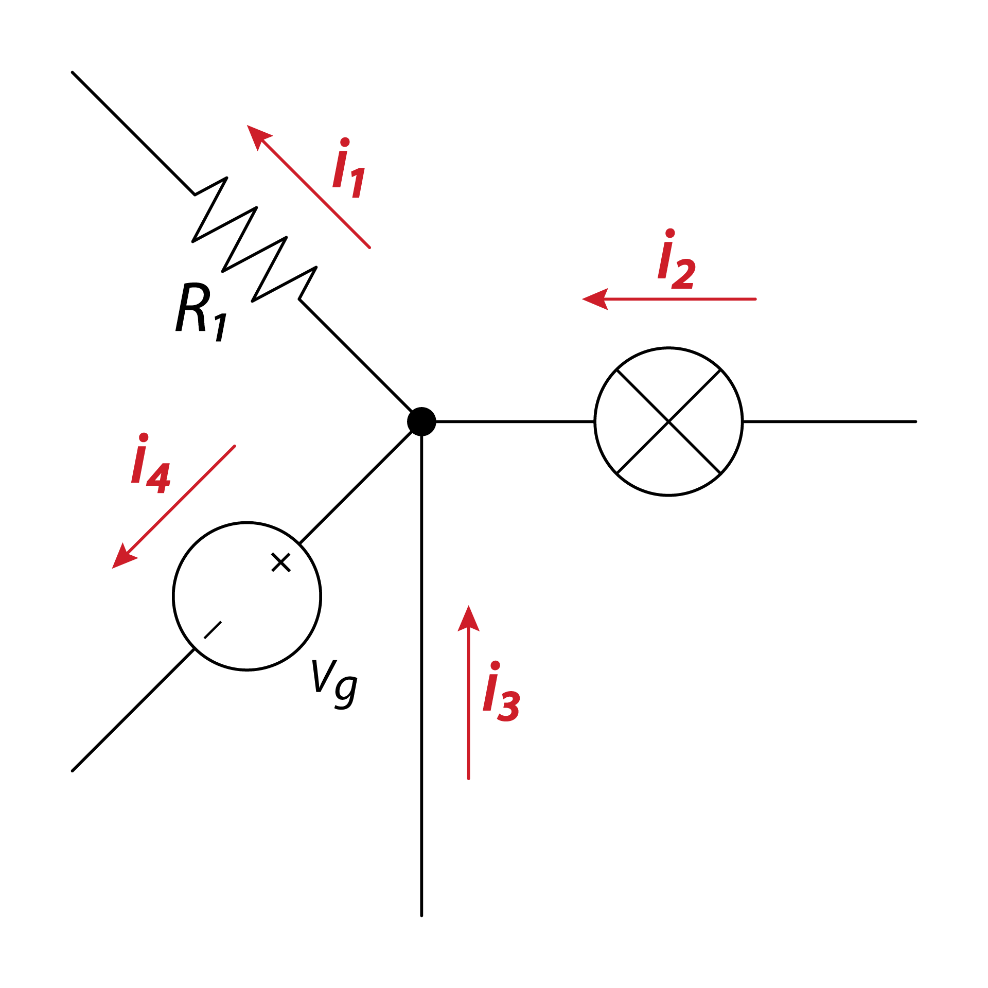
| \[i_{ 2 }+i_{ 3 }=i_{ 1 }+i_{ 4 }\] |
| \[i_{ 2 }+i_{ 3 }=i_{ 1 }+i_{ 4 }\] |
| \[i_{ 2 }+i_{ 3 }=i_{ 1 }+i_{ 4 }\] |
| \[i_{ 2 }+i_{ 3 }=i_{ 1 }+i_{ 4 }\] |
| \[i_{ 2 }+i_{ 3 }=i_{ 1 }+i_{ 4 }\] |
| Current entering any junction is equal to the current leaving that junction. Recalling that current is a signed (positive or negative) quantity reflecting direction towards or away from a node, this principle can be stated as: |
| Current entering any junction is equal to the current leaving that junction. Recalling that current is a signed (positive or negative) quantity reflecting direction towards or away from a node, this principle can be stated as: |
| Current entering any junction is equal to the current leaving that junction. Recalling that current is a signed (positive or negative) quantity reflecting direction towards or away from a node, this principle can be stated as: |
| Current entering any junction is equal to the current leaving that junction. Recalling that current is a signed (positive or negative) quantity reflecting direction towards or away from a node, this principle can be stated as: |
| Current entering any junction is equal to the current leaving that junction. Recalling that current is a signed (positive or negative) quantity reflecting direction towards or away from a node, this principle can be stated as: |
| \[\sum _{ k=1 }^{ n }{ { I }_{ k }=0 }\] |
| \[\sum _{ k=1 }^{ n }{ { I }_{ k }=0 }\] |
| \[\sum _{ k=1 }^{ n }{ { I }_{ k }=0 }\] |
| \[\sum _{ k=1 }^{ n }{ { I }_{ k }=0 }\] |
| \[\sum _{ k=1 }^{ n }{ { I }_{ k }=0 }\] |
| $n$ is the total number of branches with currents flowing towards or away from the node. This formula is valid for complex currents: |
| $n$ is the total number of branches with currents flowing towards or away from the node. This formula is valid for complex currents: |
| $n$ is the total number of branches with currents flowing towards or away from the node. This formula is valid for complex currents: |
| $n$ is the total number of branches with currents flowing towards or away from the node. This formula is valid for complex currents: |
| $n$ is the total number of branches with currents flowing towards or away from the node. This formula is valid for complex currents: |
| \[\sum _{ k=1 }^{ n }{ \tilde { I } _{ k }=0 }\] |
| \[\sum _{ k=1 }^{ n }{ \tilde { I } _{ k }=0 }\] |
| \[\sum _{ k=1 }^{ n }{ \tilde { I } _{ k }=0 }\] |
| \[\sum _{ k=1 }^{ n }{ \tilde { I } _{ k }=0 }\] |
| \[\sum _{ k=1 }^{ n }{ \tilde { I } _{ k }=0 }\] |
| The law is based on the conservation of charge whereby the charge (measured in coulombs) is the product of the current (in amperes) and the time (in seconds). |
| The law is based on the conservation of charge whereby the charge (measured in coulombs) is the product of the current (in amperes) and the time (in seconds). |
| The law is based on the conservation of charge whereby the charge (measured in coulombs) is the product of the current (in amperes) and the time (in seconds). |
| The law is based on the conservation of charge whereby the charge (measured in coulombs) is the product of the current (in amperes) and the time (in seconds). |
| The law is based on the conservation of charge whereby the charge (measured in coulombs) is the product of the current (in amperes) and the time (in seconds). |
 |
|
|
|
|
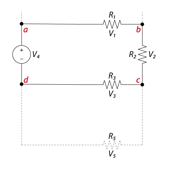
| The sum of all the voltages around a loop is equal to zero. |
| The sum of all the voltages around a loop is equal to zero. |
| The sum of all the voltages around a loop is equal to zero. |
| The sum of all the voltages around a loop is equal to zero. |
| The sum of all the voltages around a loop is equal to zero. |
| \[V_{ 1 }+V_{ 2 }+V_{ 3 }-V_{ 4 }=0\] |
| \[V_{ 1 }+V_{ 2 }+V_{ 3 }-V_{ 4 }=0\] |
| \[V_{ 1 }+V_{ 2 }+V_{ 3 }-V_{ 4 }=0\] |
| \[V_{ 1 }+V_{ 2 }+V_{ 3 }-V_{ 4 }=0\] |
| \[V_{ 1 }+V_{ 2 }+V_{ 3 }-V_{ 4 }=0\] |
| Kirchhoff’s Law for Voltage |
| Kirchhoff’s Law for Voltage |
| Kirchhoff’s Law for Voltage |
| Kirchhoff’s Law for Voltage |
| Kirchhoff’s Law for Voltage |
| Kirchhoff’s Voltage Law, also known as Kirchhoff’s second law, Kirchhoff’s loop, mesh or second rule states that the principle of the conservation of energy implies that the directed sum of the electrical potential difference (voltage) around any closed network is zero, or: More simply, the sum of the EMFS in any closed loop is equivalent to the sum of the potential drops in that loop, or: The algebraic sum of the products of the resistances of the conductors and the currents in them in a closed loop is equal to the total EMF available in that loop. Similarly to KCL, it can be stated as: |
| Kirchhoff’s Voltage Law, also known as Kirchhoff’s second law, Kirchhoff’s loop, mesh or second rule states that the principle of the conservation of energy implies that the directed sum of the electrical potential difference (voltage) around any closed network is zero, or: More simply, the sum of the EMFS in any closed loop is equivalent to the sum of the potential drops in that loop, or: The algebraic sum of the products of the resistances of the conductors and the currents in them in a closed loop is equal to the total EMF available in that loop. Similarly to KCL, it can be stated as: |
| Kirchhoff’s Voltage Law, also known as Kirchhoff’s second law, Kirchhoff’s loop, mesh or second rule states that the principle of the conservation of energy implies that the directed sum of the electrical potential difference (voltage) around any closed network is zero, or: More simply, the sum of the EMFS in any closed loop is equivalent to the sum of the potential drops in that loop, or: The algebraic sum of the products of the resistances of the conductors and the currents in them in a closed loop is equal to the total EMF available in that loop. Similarly to KCL, it can be stated as: |
| Kirchhoff’s Voltage Law, also known as Kirchhoff’s second law, Kirchhoff’s loop, mesh or second rule states that the principle of the conservation of energy implies that the directed sum of the electrical potential difference (voltage) around any closed network is zero, or: More simply, the sum of the EMFS in any closed loop is equivalent to the sum of the potential drops in that loop, or: The algebraic sum of the products of the resistances of the conductors and the currents in them in a closed loop is equal to the total EMF available in that loop. Similarly to KCL, it can be stated as: |
| Kirchhoff’s Voltage Law, also known as Kirchhoff’s second law, Kirchhoff’s loop, mesh or second rule states that the principle of the conservation of energy implies that the directed sum of the electrical potential difference (voltage) around any closed network is zero, or: More simply, the sum of the EMFS in any closed loop is equivalent to the sum of the potential drops in that loop, or: The algebraic sum of the products of the resistances of the conductors and the currents in them in a closed loop is equal to the total EMF available in that loop. Similarly to KCL, it can be stated as: |
| \[\sum _{ k=1 }^{ n }{ { V }_{ k }=0 }\] |
| \[\sum _{ k=1 }^{ n }{ { V }_{ k }=0 }\] |
| \[\sum _{ k=1 }^{ n }{ { V }_{ k }=0 }\] |
| \[\sum _{ k=1 }^{ n }{ { V }_{ k }=0 }\] |
| \[\sum _{ k=1 }^{ n }{ { V }_{ k }=0 }\] |
| Here, $n$ is the total number of voltages measured. The voltages may also be complex: |
| Here, $n$ is the total number of voltages measured. The voltages may also be complex: |
| Here, $n$ is the total number of voltages measured. The voltages may also be complex: |
| Here, $n$ is the total number of voltages measured. The voltages may also be complex: |
| Here, $n$ is the total number of voltages measured. The voltages may also be complex: |
| \[\sum _{ k=1 }^{ n }{ \tilde { V } _{ k }=0 }\] |
| \[\sum _{ k=1 }^{ n }{ \tilde { V } _{ k }=0 }\] |
| \[\sum _{ k=1 }^{ n }{ \tilde { V } _{ k }=0 }\] |
| \[\sum _{ k=1 }^{ n }{ \tilde { V } _{ k }=0 }\] |
| \[\sum _{ k=1 }^{ n }{ \tilde { V } _{ k }=0 }\] |
| This law is based on the conservation of energy whereby voltage is defined as the energy per unit charge. The total amount of energy gained per unit charge must be equal to the amount of energy lost per unit charge, as energy and charge are both conserved. |
| This law is based on the conservation of energy whereby voltage is defined as the energy per unit charge. The total amount of energy gained per unit charge must be equal to the amount of energy lost per unit charge, as energy and charge are both conserved. |
| This law is based on the conservation of energy whereby voltage is defined as the energy per unit charge. The total amount of energy gained per unit charge must be equal to the amount of energy lost per unit charge, as energy and charge are both conserved. |
| This law is based on the conservation of energy whereby voltage is defined as the energy per unit charge. The total amount of energy gained per unit charge must be equal to the amount of energy lost per unit charge, as energy and charge are both conserved. |
| This law is based on the conservation of energy whereby voltage is defined as the energy per unit charge. The total amount of energy gained per unit charge must be equal to the amount of energy lost per unit charge, as energy and charge are both conserved. |
 |
|
|
|
|
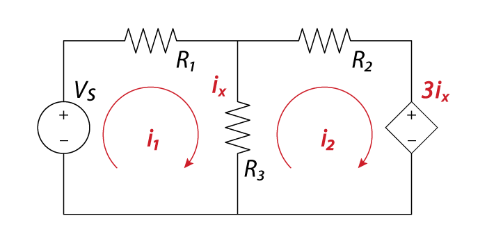
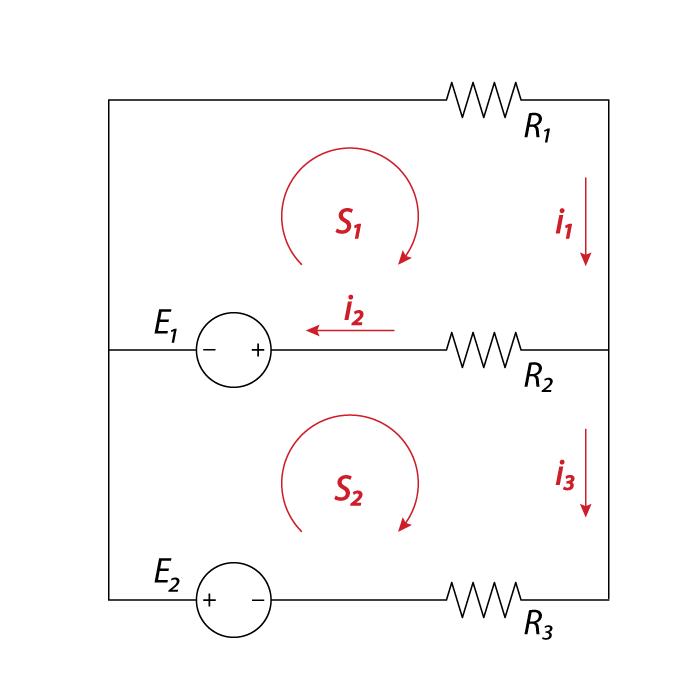
| Examples Assume an electric network consisting of two voltage sources and three resistors. According to the first law we have: |
| Examples Assume an electric network consisting of two voltage sources and three resistors. According to the first law we have: |
| Examples Assume an electric network consisting of two voltage sources and three resistors. According to the first law we have: |
| Examples Assume an electric network consisting of two voltage sources and three resistors. According to the first law we have: |
| Examples Assume an electric network consisting of two voltage sources and three resistors. According to the first law we have: |
| \[i_{ 1 }-i_{ 2 }-i_{ 3 }=0\] |
| \[i_{ 1 }-i_{ 2 }-i_{ 3 }=0\] |
| \[i_{ 1 }-i_{ 2 }-i_{ 3 }=0\] |
| \[i_{ 1 }-i_{ 2 }-i_{ 3 }=0\] |
| \[i_{ 1 }-i_{ 2 }-i_{ 3 }=0\] |
| The second law applied to the closed circuit $S_{ 1 }$ gives: |
| The second law applied to the closed circuit $S_{ 1 }$ gives: |
| The second law applied to the closed circuit $S_{ 1 }$ gives: |
| The second law applied to the closed circuit $S_{ 1 }$ gives: |
| The second law applied to the closed circuit $S_{ 1 }$ gives: |
| \[-R_{ 2 }i_{ 2 }+E_{ 1 }-R_{ 1 }i_{ 1 }=0\] |
| \[-R_{ 2 }i_{ 2 }+E_{ 1 }-R_{ 1 }i_{ 1 }=0\] |
| \[-R_{ 2 }i_{ 2 }+E_{ 1 }-R_{ 1 }i_{ 1 }=0\] |
| \[-R_{ 2 }i_{ 2 }+E_{ 1 }-R_{ 1 }i_{ 1 }=0\] |
| \[-R_{ 2 }i_{ 2 }+E_{ 1 }-R_{ 1 }i_{ 1 }=0\] |
| The second law applied to the closed circuit $S_{ 2 }$: |
| The second law applied to the closed circuit $S_{ 2 }$: |
| The second law applied to the closed circuit $S_{ 2 }$: |
| The second law applied to the closed circuit $S_{ 2 }$: |
| The second law applied to the closed circuit $S_{ 2 }$: |
| \[-R_{ 3 }i_{ 3 }-E_{ 2 }-E_{ 1 }+R_{ 2 }i_{ 2 }=0\] |
| \[-R_{ 3 }i_{ 3 }-E_{ 2 }-E_{ 1 }+R_{ 2 }i_{ 2 }=0\] |
| \[-R_{ 3 }i_{ 3 }-E_{ 2 }-E_{ 1 }+R_{ 2 }i_{ 2 }=0\] |
| \[-R_{ 3 }i_{ 3 }-E_{ 2 }-E_{ 1 }+R_{ 2 }i_{ 2 }=0\] |
| \[-R_{ 3 }i_{ 3 }-E_{ 2 }-E_{ 1 }+R_{ 2 }i_{ 2 }=0\] |
| Thus we get a linear system of equations in $i_{ 1 }$, $i_{ 2 }$, and $i_{ 3 }$: |
| Thus we get a linear system of equations in $i_{ 1 }$, $i_{ 2 }$, and $i_{ 3 }$: |
| Thus we get a linear system of equations in $i_{ 1 }$, $i_{ 2 }$, and $i_{ 3 }$: |
| Thus we get a linear system of equations in $i_{ 1 }$, $i_{ 2 }$, and $i_{ 3 }$: |
| Thus we get a linear system of equations in $i_{ 1 }$, $i_{ 2 }$, and $i_{ 3 }$: |
| \[\begin{cases} i_{ 1 }-i_{ 2 }-i_{ 3 }=0 \\ -R_{ 2 }i_{ 2 }+E_{ 1 }-R_{ 1 }i_{ 1 }=0 \\ -R_{ 3 }i_{ 3 }-E_{ 2 }-E_{ 1 }+R_{ 2 }i_{ 2 }=0 \end{cases}\] |
| \[\begin{cases} i_{ 1 }-i_{ 2 }-i_{ 3 }=0 \\ -R_{ 2 }i_{ 2 }+E_{ 1 }-R_{ 1 }i_{ 1 }=0 \\ -R_{ 3 }i_{ 3 }-E_{ 2 }-E_{ 1 }+R_{ 2 }i_{ 2 }=0 \end{cases}\] |
| \[\begin{cases} i_{ 1 }-i_{ 2 }-i_{ 3 }=0 \\ -R_{ 2 }i_{ 2 }+E_{ 1 }-R_{ 1 }i_{ 1 }=0 \\ -R_{ 3 }i_{ 3 }-E_{ 2 }-E_{ 1 }+R_{ 2 }i_{ 2 }=0 \end{cases}\] |
| \[\begin{cases} i_{ 1 }-i_{ 2 }-i_{ 3 }=0 \\ -R_{ 2 }i_{ 2 }+E_{ 1 }-R_{ 1 }i_{ 1 }=0 \\ -R_{ 3 }i_{ 3 }-E_{ 2 }-E_{ 1 }+R_{ 2 }i_{ 2 }=0 \end{cases}\] |
| \[\begin{cases} i_{ 1 }-i_{ 2 }-i_{ 3 }=0 \\ -R_{ 2 }i_{ 2 }+E_{ 1 }-R_{ 1 }i_{ 1 }=0 \\ -R_{ 3 }i_{ 3 }-E_{ 2 }-E_{ 1 }+R_{ 2 }i_{ 2 }=0 \end{cases}\] |
| Which is equivalent to: |
| Which is equivalent to: |
| Which is equivalent to: |
| Which is equivalent to: |
| Which is equivalent to: |
| \[\begin{cases} i_{ 1 }+-i_{ 2 }+-i_{ 3 }=0 \\ R_{ 1 }i_{ 1 }+R_{ 2 }i_{ 2 }+0i_{ 3 }=E_{ 1 } \\ 0i_{ 1 }+R_{ 2 }i_{ 2 }-R_{ 3 }i_{ 3 }=E_{ 1 }+E_{ 2 } \end{cases}\] |
| \[\begin{cases} i_{ 1 }+-i_{ 2 }+-i_{ 3 }=0 \\ R_{ 1 }i_{ 1 }+R_{ 2 }i_{ 2 }+0i_{ 3 }=E_{ 1 } \\ 0i_{ 1 }+R_{ 2 }i_{ 2 }-R_{ 3 }i_{ 3 }=E_{ 1 }+E_{ 2 } \end{cases}\] |
| \[\begin{cases} i_{ 1 }+-i_{ 2 }+-i_{ 3 }=0 \\ R_{ 1 }i_{ 1 }+R_{ 2 }i_{ 2 }+0i_{ 3 }=E_{ 1 } \\ 0i_{ 1 }+R_{ 2 }i_{ 2 }-R_{ 3 }i_{ 3 }=E_{ 1 }+E_{ 2 } \end{cases}\] |
| \[\begin{cases} i_{ 1 }+-i_{ 2 }+-i_{ 3 }=0 \\ R_{ 1 }i_{ 1 }+R_{ 2 }i_{ 2 }+0i_{ 3 }=E_{ 1 } \\ 0i_{ 1 }+R_{ 2 }i_{ 2 }-R_{ 3 }i_{ 3 }=E_{ 1 }+E_{ 2 } \end{cases}\] |
| \[\begin{cases} i_{ 1 }+-i_{ 2 }+-i_{ 3 }=0 \\ R_{ 1 }i_{ 1 }+R_{ 2 }i_{ 2 }+0i_{ 3 }=E_{ 1 } \\ 0i_{ 1 }+R_{ 2 }i_{ 2 }-R_{ 3 }i_{ 3 }=E_{ 1 }+E_{ 2 } \end{cases}\] |
| Assuming: |
| Assuming: |
| Assuming: |
| Assuming: |
| Assuming: |
| \[R_{ 1 }=100,\quad R_{ 2 }=200,\quad R_{ 3 }=300\quad (ohms);\quad E_{ 1 }=3,\quad E_{ 2 }=4\quad (volts)\] |
| \[R_{ 1 }=100,\quad R_{ 2 }=200,\quad R_{ 3 }=300\quad (ohms);\quad E_{ 1 }=3,\quad E_{ 2 }=4\quad (volts)\] |
| \[R_{ 1 }=100,\quad R_{ 2 }=200,\quad R_{ 3 }=300\quad (ohms);\quad E_{ 1 }=3,\quad E_{ 2 }=4\quad (volts)\] |
| \[R_{ 1 }=100,\quad R_{ 2 }=200,\quad R_{ 3 }=300\quad (ohms);\quad E_{ 1 }=3,\quad E_{ 2 }=4\quad (volts)\] |
| \[R_{ 1 }=100,\quad R_{ 2 }=200,\quad R_{ 3 }=300\quad (ohms);\quad E_{ 1 }=3,\quad E_{ 2 }=4\quad (volts)\] |
| The solution is: |
| The solution is: |
| The solution is: |
| The solution is: |
| The solution is: |
| \[\begin{cases} i_{ 1 }=\frac { 1 }{ 1100 } \\ i_{ 2 }=\frac { 4 }{ 275 } \\ i_{ 3 }=\frac { 3 }{ 220 } \end{cases}\] |
| \[\begin{cases} i_{ 1 }=\frac { 1 }{ 1100 } \\ i_{ 2 }=\frac { 4 }{ 275 } \\ i_{ 3 }=\frac { 3 }{ 220 } \end{cases}\] |
| \[\begin{cases} i_{ 1 }=\frac { 1 }{ 1100 } \\ i_{ 2 }=\frac { 4 }{ 275 } \\ i_{ 3 }=\frac { 3 }{ 220 } \end{cases}\] |
| \[\begin{cases} i_{ 1 }=\frac { 1 }{ 1100 } \\ i_{ 2 }=\frac { 4 }{ 275 } \\ i_{ 3 }=\frac { 3 }{ 220 } \end{cases}\] |
| \[\begin{cases} i_{ 1 }=\frac { 1 }{ 1100 } \\ i_{ 2 }=\frac { 4 }{ 275 } \\ i_{ 3 }=\frac { 3 }{ 220 } \end{cases}\] |
| $i_{ 3 }$ has a negative sign, denoting the direction of $i_{ 3 }$ as opposite to the assumed direction. |
| $i_{ 3 }$ has a negative sign, denoting the direction of $i_{ 3 }$ as opposite to the assumed direction. |
| $i_{ 3 }$ has a negative sign, denoting the direction of $i_{ 3 }$ as opposite to the assumed direction. |
| $i_{ 3 }$ has a negative sign, denoting the direction of $i_{ 3 }$ as opposite to the assumed direction. |
| $i_{ 3 }$ has a negative sign, denoting the direction of $i_{ 3 }$ as opposite to the assumed direction. |
Discovered in 1845 by Gustav Robert Kirchhoff. |
Discovered in 1845 by Gustav Robert Kirchhoff. |
Discovered in 1845 by Gustav Robert Kirchhoff. |
Discovered in 1845 by Gustav Robert Kirchhoff. |
Discovered in 1845 by Gustav Robert Kirchhoff. |